The relationship between the Average Deal Price of Shanghai License Plate and the Number of Bidders

1 Hypothesis

Increasing in the average deal price of Shanghai license plate will increase the number of bidders.

2 Data Exploration

2.1        Background

Over the last two decades, there is an increase in automobile ownership and use in China. This increases energy consumption, worsens air pollution and exacerbates congestion. Therefore, an auction system has been adopted by Shanghai government to limit the number of license plates issued for every month.

The dataset contains monthly auction data from Jan 2002 to Oct 2017. Feb 2008 data is missing, and the number of records is 189 [1].

2.2        Metadata

Field	Description	Data Type
Date	Jan 2002 to Oct 2017 (Feb 2008 is missing)	Date
avg_deal_price	The average deal price of Shanghai license plate	Numeric
lowest_deal_price	The lowest deal price of Shanghai license plate	Numeric
num_bidder	Number of citizens who participate the auction for the month	Numeric
num_plates	number of plates that will be issued by the government for the month	Numeric

Table 1 Metadata

Only variables “avg_deal_price” and “num_bidder” will be analysed in this report.

 

3          Transfer Function Modelling

Assuming that the relationship between “avg_deal_price” and “num_bidder” is unidirectional, JMP is used for the analysis. Since the hypothesis is increasing in the average deal price of Shanghai license plate will increase the number of bidders, so taking “avg_deal_price” as the input and “num_bidder” as the output.

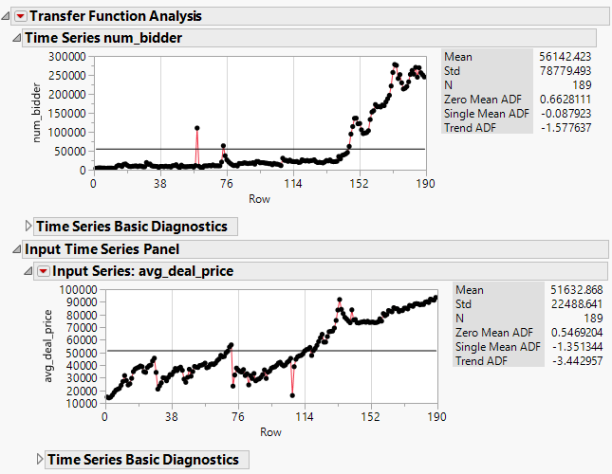
Figure 1 Time series plot of input and output variables

Figure 1 shows that the trends of input and output are both not stationary, so an order 1 differencing is applied to both input and output.

Figure 2 Plot of Input with order 1 differencing

Figure 3 Plot of output with order 1 differencing

 

Then the trends of input and output become stationary.

Figure 4 Autocorrelation and partial autocorrelation graphs

Since there is no seasonality observed, so ARIMA instead of seasonal ARIMA is applied next to both input and output. Figure 4 shows that there is a distinct drop in the Partial autocorrelation function (PACF) value after lag 3, an AR(3) model is plotted.

Figure 5 AR(3) Model for input

However, Figure 5 shows that the values for AR2 and AR3 in Column Prob>|t| are big. Therefore, AR(1) model is adopted for both input and output instead of AR(3).

Figure 6 AR(1) Model for input

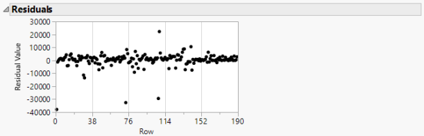
Figure 7 Residuals of AR(1) model for input

Figure 8 AR(1) Model for output

Figure 9 Residuals of AR(1) model for output

Figure 7 and Figure 9 show that the residuals of AR(1) models for both input and output are random.

Next, in order to remove the autocorrelation, pre-whitening is performed to the input variable.

Figure 10 Pre-whitening plot for dataset from Jan 2002 to Oct 2017

Figure 10 shows that there is an increase in the values at both negative lag (lag -14 and -13) and positive lag (lag 1 and 2). This means the cross-correlation is bi-directional. Therefore, the cointegration technique needs to be applied.

 

4          Bi-Directional Cross-Correlation Analysis

Since the cross-correlation is bi-directional, cointegration analysis with GRETL is performed.

Firstly, a time series plot of both variables is plotted as shown in Figure 11. It shows that both variables values are increasing gradually from the Year 2002 to 2014. Then from the Year 2014 to 2016, there is a big increase in “num_bidder”, but “avg_deal_price” increases in a similar rate as previous years.

Figure 11 Time series plot of both variables from Jan 2002 to Oct 2017

Then the Engle-Graner test for cointegration is performed and the steps are,

Step 1: Determine ‘d’ in I(d) for the first series, where d represents the order of integration and is abbreviated I(d). d is the number of times the series has to be different to be made stationary. ADF unit root test is used to determine d.

Step 2: Determine ‘d’ in I(d) for the second series

Step 3: Estimate cointegration regression: Y_t = β₁ + β₂X_t + ε_t

Step 4: Determine ‘d’ in I(d) for ε_t

                                H₀: Unit root (i.e., not cointegrated)

H_A: No unit root (i.e., cointegrated)

To perform the ADF unit root test on the residuals from the cointegrating regression to determine the order of integration [2].

 

4.1        Step 1: Determine ‘d’ in I(d) for the first series

Augmented Dickey-Fuller (ADF) test is performed in Step 1 for series “avg_deal_price”. Taking 6 as the lag order for ADF test which is the cube root of the data size which is 189.

Figure 12 ADF test for series “avg_deal_price”

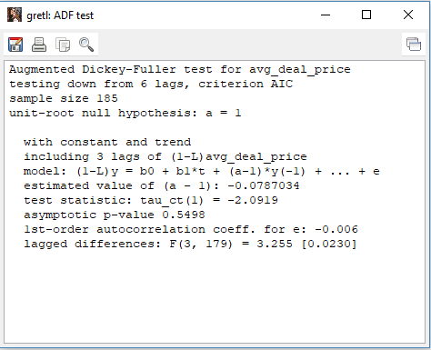
Figure 13 ADF test result for series “avg_deal_price”

Figure 13 shows that the p-value is 0.5498 which is large, hence fail to reject the null hypothesis. Therefore, the series needs to be different to make it stationary. d=1 for “avg_deal_price”.

 

4.2        Step 2: Determine ‘d’ in I(d) for the second series

The same test is done for series “num_bidder”. Figure 14 shows the p-value is 0.9175 which is large, hence fail to reject the null hypothesis. Therefore, the series needs to be different to make it stationary. d=1 for “num_bidder”.

Figure 14 ADF test for series “num_bidder”

 

4.3        Step 3 and Step 4

The Engle-Graner cointegration test is performed, taking “avg_deal_price” as the independent variable and “num_bidder” as the dependent variable. Figure 15 shows the result that the p-value is 0.2498 which is not small, hence fail to reject the null hypothesis at 5% level of significance. This means there is no cointegration relation between the two variables.

Figure 15 Engle-Graner cointegration test result for dataset from Jan 2002 to Oct 2017

 

5          Further Exploration

Since Figure 11 shows that there is a big increase in “num_bidder”, but “avg_deal_price” still increase gradually, this may be the reason that the relationship between two variables is neither unidirectional nor bi-directional. Therefore, data from Jan 2002 to Dec 2013 is going to be analysed instead.

Figure 16 Time series plot of both variables from Jan 2002 to Dec 2013

Firstly, use JMP to perform the unidirectional relationship analysis between two variables as mentioned in Section 3. The result as shown in Figure 17 shows that the cross-correlation is bi-directional. Therefore, GRETL is used to perform bi-directional cross-correlation analysis.

Figure 17 Pre-whitening plot for dataset from Jan 2002 to Dec 2013

Since the number of records is 143, so taking 6 as the lag order for ADF test which is the cube root of the data size which is 143. Following the same steps mentioned in Section 4, the Engle-Graner cointegration test result is shown in Figure 18.

Figure 18 Engle-Graner cointegration test result for dataset from Jan 2002 to Dec 2013

The result shows the p-value is 4.709e^-13 which is small, so reject the null hypothesis at 5% level of significance. This means there is cointegration relation between two variables and the series can be written as an error correction model.

Equation 1 Error correction model equation

Equation 1 shows the equation of the error correction model. The residuals from the cointegrating regression are found within the brackets and capture the departure from the attractor from last period. The coefficient gamma is the speed of adjustment, if it is not statistically significant, the variable is weakly exogenous. Before estimating the error correction model, the cointegrating regression is estimated and the residuals are saved.

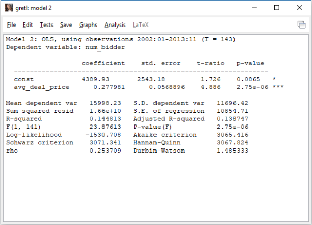
Figure 19 Ordinary least squares method result

Ordinary least squares method is performed to save the residuals. After the residuals are saved, two new series “d_avg_deal_price” and “d_num_bidder” are created that are the difference of the “avg_deal_price” and “num_bidder” as shown in Figure 20. Next step is to estimate the error correction model.

Figure 20 New variables are created

Figure 21 Adding lags

Figure 22 Ordinary least squares method with new variables lagged by 1

To estimate the error correction model, ordinary least squares is applied as shown in Figure 22. The variables are lagged by 1 and remove the “const” is removed.

Figure 23 Ordinary least squares method result with new variables

The p-value of variable e_1 is 8.81e^-10 which is statistically significant. This means the dependent variable “num_bidder” is not weakly exogenous and moves to restore the equilibrium when the system is out of balance.

 

6          Conclusion

From the Year 2014 to 2016, there is a big increase in the number of bidders, but the average deal price of Shanghai license plate increases at a similar rate as previous years. This may be the reason that the relationship between the average deal price of Shanghai license plate and the number of bidders is neither unidirectional nor bi-directional from Jan 2002 to Oct 2017.

However, from Jan 2002 to Dec 2013, there is a bi-directional cross-correlation between the average deal price of Shanghai license plate and the number of bidders. The number of bidders is not weakly exogenous and moves to restore the equilibrium when the system is out of balance.

 

7          References

[1] “Shanghai license plate bidding price prediction,” 2017. [Online]. Available: https://www.kaggle.com/bazingasu/shanghai-license-plate-bidding-price-prediction.
[2] Janelle, “Cointegration (Video 7 of 7 in the gretl Instructional Video Series),” 17 Feb 2015. [Online]. Available: https://www.youtube.com/watch?v=bJgx3JLb7fI&t=311s.

 

To Predict the Concentration of Atmospheric Particulate Matter in Northern Taiwan by Multiple Linear Regression

1. Introduction

An air quality monitoring dataset for Northern Taiwan was obtained from the Environmental Protection Administration of Taiwan. This dataset contains measurements from 25 observation stations located in Northern Taiwan, and comprises of 21 meteorological and environmental parameters measured in 2015.

2. Objective

The aim of this report is to build a predictive model using Multiple Linear Regression to predict the concentration of atmospheric particulate matter with diameter less than 2.5 micrometer (PM2.5) based on other measured environmental and meteorological data.

3. Data Preparation

Prior to using the dataset for analysis, a series of data preparation activities were carried out. This includes a sanity check of the data reported for each variable to ensure that the range of values reported for each variable were logical. The steps involved in data preparation are detailed in the following sub sections.

3.1 Invalid values

As identified in the data dictionary (included in the Appendix), invalid values due to equipment inspection, program inspection and human inspection were appended with “#,* and x” respectively. As these values could not be imputed reliably, listwise deletion was used to remove all rows containing such invalid values.

3.2 Data Imputation

As indicated in the data dictionary, three variables (PH_RAIN, RAINFALL and RAIN_COND) had “NR” (No Rainfall) indicated. While those under RAINFALL could be imputed as “0”, as no rainfall means that 0mm of rainfall was measured, such observations under PH_RAIN and RAIN_COND had to be removed, as it’s not possible to reflect these values numerically.

3.3 Removal of Date/Time and Location

Considering that the 21 environmental variables contains information such as humidity, ambient temperature etc, it was determined that these variables were sufficient to describe the conditions of the location and the time at which these data were collected. As such, Date/Time and Location were excluded in our analysis.

3.4 Missing Values

The remaining observations which had missing values after the above steps were removed due to the lack of domain knowledge. It was decided that imputation without the necessary domain knowledge may skew the dataset, and make the modelling less accurate.

4. Multiple Linear Regression Model Building

4.1 Visual Inspection of the Scatterplot of PM2.5

Figure 1: Scatterplot of PM2.5 versus all other variables

After data preparation was completed, a scatterplot of PM2.5 against all other variables was generated to investigate if there is any evidence of linearity between other predictors. From Figure 1, its noted that there’s a very strong evidence of linearity between PM10 and PM2.5. This is logical, because the definition of PM10 (Particulate Matter of less than 10 micrometer in diameter) also overlaps the definition of PM2.5. Apart from this, PH_RAIN and NO₂ also appears to be following the trend of the fitted line generated. As such, this dataset was deemed suitable for Multiple Linear Regression.

4.2 Approach

To investigate if the 20 variables are sufficiently significant in explaining the variance of the dataset, these variables would be used in model fitting with their p values evaluated against a level of significance of 0.05, and the adjusted R² reviewed. Once the predictors have been finalized, their Variance Inflationary Factor (VIF) would be checked to ensure that no multi-collinearity exists between themselves.

4.3 Training and Validation Data Split

After the Data Preparation stage, the final dataset contains a total of 583 samples with 1 target variable and 20 predictors. Considering that the number of observations versus the number of predictors exceed the 10:1 ratio, the size of the dataset was deemed sufficient for Multiple Linear Regression. The dataset was then split into training data and test data based on a ratio of 70:30, so that sufficient data was available to train and validate the model.

4.4 Training Data Model

4.4.1 Model Building

From the training dataset obtained in section 4.3, a linear model was fitted with PM2.5 set as the dependent variable. Based on the results generated in R, the least significant variable was iteratively dropped, with the model evaluated after each removal of variables. This process was completed once there were no insignificant variables remaining.

Table 1: Removal of Variables and Resulting Adjusted R²

Sequence of Removal	Variable Dropped	Adjusted R²
initial model	–	0.8106
1	NO	0.8111
2	NMHC	0.8116
3	RAINFALL	0.812
4	RAIN_COND	0.8125
5	WIND_SPEED	0.8128
6	WIND_DIREC	0.813
7	CH4	0.8129
8	NO2	0.8122
9	THC	0.8117
10	WD_HR	0.8112
11	NOx	0.8105

The significant variables remaining are listed in Table 2. At this stage, the adjusted R² of the model is 0.8105. In addition, by inspecting the values of Estimate ± Standard Error, it’s verified that the coefficients of these variables are non-zero. As such, the finalised variables are considered sufficient for further analysis.

Table 2: List of Variables, Estimate, Standard Error and P Value

Variable	Interpretation	Estimate	Standard Error	P value
AMB_TEMP	Ambient Air Temperature	-0.24038	0.04669	0.000000414
CO	Carbon Monoxide	4.93266	0.93706	0.000000231
O3	Ozone	0.06573	0.02042	0.001388
PH_RAIN	pH of Rain	-1.35644	0.34374	0.0000938
PM10	Particulate Matter ≤ 10µm	0.47179	0.01566	< 2e-16
RH	Relative Humidity	0.18825	0.04953	0.000167
SO2	Sulphur Dioxide	0.40099	0.18984	0.035289
UVB	Ultraviolet B	0.66109	0.29199	0.024104
WS_HR	Average Wind Speed per Hour	-0.59653	0.17656	0.0008

4.4.2 Residual Analysis

Figure 2: Diagnostic Plots for Linear Regression Analysis

4.4.2.1 Non-Linearity between Dependent and Predictor Variables

From Figure 2, it’s observed from the Residuals versus Fitted Plot that there is no non-linear relationship between the predictors and the dependent variable. This means that the multiple linear regression model is capable of capturing the data in the trained dataset.

4.4.2.2 Normality of Residuals

From the Normal Q-Q Plot, a straight line is observed. This satisfies the assumption that the residuals are normally distributed.

4.4.2.3 Homoscedasticity of Residuals

From the Scale-Location Plot, there appears to be evidence of heteroscedasticity, as the red line is moving upwards as the fitted values increases beyond 30. Further verification through the Breusch-Pagan Test in R confirms that heteroscedasticity is present, with a p-value of less than 2.2e-16. This violates the assumption of linear regression that the variance of the residuals is constant.

4.4.2.4 Effect of Outliers on Model

Lastly, the Residuals versus Leverage Plot indicates that there are no outliers that have a high Cook’s distance. This means that any outliers in our dataset, if any, are not significant in influencing the linear regression model built.

4.4.3 Correcting the model for Heteroscedasticity

Since heteroscedasticity is observed in our model as indicated in section 4.4.2.3, transformation of the dependent variable and application of a weighted least squares model were two approaches explored in an attempt to correct the model.

4.4.3.1 Dependent Variable Transformation

Various approaches (e.g. applying a natural logarithmic function to PM2.5) were explored to transform the dependent variable before rebuilding a new model. However, the approach that yielded the best result appeared to be a Box Cox Transformation. The intent of Box Cos Transformation is to find a value of λ such that the dependent variable is transformed to the following:Due to the limitation of the transformation, 13 instances of the training dataset where PM2.5 = 0 was removed. Based on the transformation, λ = 0.4 was obtained. Building a new model based on this new transformed dependent variable yielded the results in Table 3, with an adjusted R² of 0.7577.

Table 3: List of Variables, Estimate, Standard Error and P Value (Transformed Dependent Variable)

Variable	Interpretation	Estimate	Standard Error	P value
AMB_TEMP	Ambient Air Temperature	-0.05957	0.009197	2.82E-10
CO	Carbon Monoxide	0.76531	0.3363	0.02341
NMHC	Non-Methane Hydrocarbon	1.38527	0.65308	0.03454
O3	Ozone	0.01689	0.00424	8.2E-05
PH_RAIN	pH of Rain	-0.3407	0.07574	9.1E-06
PM10	Particulate Matter ≤ 10µm	0.08149	0.00337	< 2E-16
SO2	Sulphur Dioxide	0.08564	0.04279	0.04606
WS_HR	Average Wind Speed per Hour	-0.1588	0.04859	0.00118

Figure 3: Diagnostic Plots for Linear Regression Analysis (Transformed Dependent Variable)

On inspecting the residual diagnostic plots of the newly built model, it’s noted that there is an improvement in the Scale-Location Plot. In addition, the characteristics of the other three plots remain unchanged. However, on verifying the model with the Breusch -Pagan Test, it’s noted that the residuals are still considered as heteroscedastic, with a p-value of 4.766e-08 rejecting the null hypothesis that the residuals are homoscedastic.

4.4.3.2 Weighted Least Squares

Since the initial model was built based on ordinary least square estimators, heteroscedasticity was likely to occur due to incorrect computation of standard errors. Accordingly, the initial model was transformed into one with homoscedastic errors, using generalized least squares estimator.

It is noted that this transformation requires a logarithmic function to be applied on all predictors. As such, observations wherein the variables contained zero value were removed (2 occurrences of SO2 and 1 occurrence of WS_HR), while UVB was removed from the dataset altogether as there were 233 occurrences of zero values for this variable, amounting to more than half of the training dataset. This resulted in a training dataset of 407 observations with 19 variables used to build a new model applying weighted least squares.

The fitted models are as follows:

Ordinary Least Squares:

Generalised Least Squares:

However, the adjusted R² of the Generalised Least Squares model dropped from 0.8105 to 0.8047, while the p-value of the Breusch-Pagan Test did not improve. Hence, this approach was not considered to be appropriate, and the dependent variable transformation approach was adopted instead. 

4.5 Multi-Collinearity

Based on the model built in section 4.4.3.1, a VIF test was done to inspect the finalized dataset for multi-collinearity.

Table 4: VIF Results

AMB_TEMP	CO	NMHC	O3	PH_RAIN	PM10	SO2	WS_HR
1.200704	5.088495	5.868661	1.933892	1.282449	1.304998	1.247557	1.276881

From the results, it was noted that CO and NMHC exhibit multi-collinearity against each other. NMHC was dropped due to its lower significance compared to CO, resulting in a model without multi-collinearity. At this point, the adjusted R² is 0.7556, which is a negligible drop from the earlier model. In addition, the residual diagnostic plots did not exhibit any difference due to the removal of NMHC from the model.

4.6 Model Accuracy

With the model finalized, the validation dataset was used to evaluate the prediction accuracy of the model. Predicted values of the transformed dependent variables were generated with λ = 0.4 as per section 4.4.3.1, and these were compared with the actual values of the transformed dependent variables using the Mean Absolute Percentage Error (MAPE).

The formula of MAPE is given by:where n is number of observations,  is the actual value, and  is the forecasted value.

Since the limitation of MAPE is that Actual values cannot be zero (due to division by 0), these two occurrences were removed from the test dataset first. This gives us a MAPE of 25.8%. While this result is not ideal, there’s a marked improvement in accuracy as compared to the original model built in section 4.1, before dependent variable transformation. If that model was used, the MAPE of that model comes to 34.3%. 

5. Final Model

The formula of the final model is given by:

6. Conclusion

In this report, an air quality monitoring dataset for Northern Taiwan was used to build a Multiple Linear Regression model to predict the concentration of PM2.5 based on other measured environmental and meteorological data. While the dataset was assessed to be suitable for Linear Regression, heteroscedasticity of the residuals was observed during the initial residual analysis. The dependent variable was transformed using Box Cox Transformation to correct for heteroscedasticity, resulting in an approximately 10% improvement in model accuracy as compared to the original approach, with the final model having a MAPE of 25.8% based on the validation dataset. Moving forward, an alternative predictive model such as logistic regression through categorizing PM2.5 into dichotomous levels (e.g. Healthy, Unhealthy) could be explored to improve the accuracy of the predictive model, as homoscedasticity is not required for error terms in logistic regression.

Appendix A

The following metadata is provided by the Environmental Protection Administration of Taiwan together with the raw data.

The columns in csv file are:

• time – The first column is observation time of 2015
• station – The second column is station name, there is 25 observation stations
  • [Banqiao, Cailiao, Datong, Dayuan, Guanyin, Guting, Keelung, Linkou, Longtan, Pingzhen, Sanchong, Shilin, Songshan, Tamsui, Taoyuan, Tucheng, Wanhua, Wanli, Xindian, Xinzhuang, Xizhi, Yangming, Yonghe, Zhongli, Zhongshan]
• items – From the third column to the last one
  • item – unit – description
  • SO2 – ppb – Sulfur dioxide
  • CO – ppm – Carbon monoxide
  • O3 – ppb – ozone
  • PM10 – μg/m3 – Particulate matter
  • 5 – μg/m3 – Particulate matter
  • NOx – ppb – Nitrogen oxides
  • NO – ppb – Nitric oxide
  • NO2 – ppb – Nitrogen dioxide
  • THC – ppm – Total Hydrocarbons
  • NMHC – ppm – Non-Methane Hydrocarbon
  • CH4 – ppm – Methane
  • UVB – UVI – Ultraviolet index
  • AMB_TEMP – Celsius – Ambient air temperature
  • RAINFALL – mm
  • RH – % – Relative humidity
  • WIND_SPEED – m/sec – The average of last ten minutes per hour
  • WIND_DIREC – degress – The average of last ten minutes per hour
  • WS_HR – m/sec – The average of hour
  • WD_HR – degress – The average of hour
  • PH_RAIN – PH – Acid rain
  • RAIN_COND – μS/cm – Conductivity of acid rain

Data mark

• # indicates invalid value by equipment inspection
• indicates invalid value by program inspection
• x indicates invalid value by human inspection
• NR indicates no rainfall
• blank indicates no data

 

Team members:

Student ID	Name
A0178551X	Choo Ming Hui Raymond
A0178431A	Huang Qingyi
A0178415Y	Jiang Zhiyuan
A0178365R	Wang Jingli
A0178500J	Yang Chia Lieh

Causes and effects of ageing population in Singapore.

Introduction

The ageing population in Singapore increasing in a faster rate which seems to be a threat to Singapore.There are many causes for this increase in the ageing population. There are large number of unmarried people and the steady decline in fertility rate over the years and increase in number of people getting divorced and higher life expectancy at birth.The effect of having a larger number of elderly people impacts the GDP of the nation in the coming years .This can also increase the  demand for more doctors and healthcare professionals as well as the need for more technologies pertaining to healthcare.

Goal

Our goal is the study the population trend in Singapore and the factors affecting the population and how it affects the economy of the country.

Scope of the study

This presentation is useful to the govt officials in the Ministry of manpower to give them an insight on how the GDP is related to the ageing population in Singapore.This dashboard also portrays various metrics such as fertility rate,divorce rate,no of singles and their impact in ageing population.So based on our dashboard we can take suggest some useful measures that can improve the economy by promoting healthy trends that increases the population of  Singapore.

Questions

What is the trend in the population of unmarried people in the last ten years?

The population of unmarried singles is fluctuating ,but the data shows that the population of unmarried singles have come slightly down. This is a healthy trend.

Is the present divorce rate more than the previous year?

The divorce rates are going up ,which eventually leads to lack of babies and children being abandoned. This is an unhealthy trend

Does decrease in fertility rate increase the ageing population of Singapore?

The decrease in fertility rate leads to decrease in population ,the ageing population sustains and grow weaker and thus leads to shortage of skilled workers.

Does higher life expectancy at birth increase the median age of Singapore?

The average life expectancy is above 80 years ,which is an increase compared to the previous years.As the fertility rate is low,the high life expectancy can increase the median age of the population (currently it is 45).Source:singstat.gov.sg

Does ageing population cause a demand for more doctors?

The ageing population of Singapore can increase the demand for more healthcare professionals. Singapore has a significant population of old people affected by Parkinson’s disease and Alzeimers .Hence more physiotherapists and technologies for assisting the aged are in demand

Does working population of Singapore impact the GDP?

The present GDP of Singapore is 52,960.71USD.As the population ages with time ,the people entering the workforce is lesser than the people exiting the workforce. This imbalanced nature of supply vs demand impacts the economy and hence the GDP.

 

METRICS

1. Annual fertility rate .
2. Median age of population
3. Average life expectancy
4. Divorce rates per year
5. Singles count per year.

 

DASHBOARD

INSIGHTS

1.

From the above scorecard ,it is found that the increase in working population contributes more to the GDP of the country.

2.

From the above scorecard ,the fertility rate decreases with the increase in the  count of singles.

CONCLUSION

It is clear that the population will sharp decline at a particular point of time which will have a negative impact in the GDP of the nation. The ageing population also demands for more number of Doctors, Nurse and Hospitals in the coming years. So it indicates that there is a strong need for more young people to be in the workforce. The fertility rate has to be increased as it is the only way to promote population growth.

 

DATA SOURCES

1.www.singstat.gov.sg/docs/default…/population

2 .www.population.sg/population-trends/demographics

3.https://www.nptd.gov.sg/PORTALS/0/HOMEPAGE/…/population-in-brief-2016.pdf

4.https://data.gov.sg/dataset/resident-population-by-ethnicity-gender-and-age-group

5. http://www.straitstimes.com/singapore/rapid-ageing-a-pressing-issue

6. http://www.todayonline.com/singapore/singapore-feeling-impact-rapidly-ageing-population

 

TEAM MEMBERS

SHIVARAM ANDIAPPAN SELVARAJ

ARUN SUGUMAR GURUMOORTHY

JOSEPH PABLO VARUN

PRAVEEN GUDDALA KUMARAN

 

 

 

 

 

 

Healthcare Manpower Shortage in next 10 Years

With the rapid growth of aging population and chronic diseases, the health system of Singapore is now facing great challenge: a serious shortage of healthcare manpower. The shortage of doctors or nurses will probably lead to decreasing quality of healthcare provided and increasing healthcare costs. The team is to present the dashboard on healthcare workforce to the Director of Manpower Development of Ministry of Health to address the issue of shortage.

Goal

To explore options to meet the rising demand for healthcare in Singapore over the next 10 years

Questions

1. How has the demand for healthcare changed since 2000?
2. What will the demand for healthcare be like 10 years from now?
3. How has the Healthcare workforce meeting this demand?
4. Will the healthcare workforce be able to continue meeting the demand for healthcare 10 years from now?
5. How does the proportion of doctors in Singapore compare with other countries?
6. What strategies can we take to increase the healthcare workforce in Singapore?

Metrics

• Hospitals and polyclinics admissions over time
• Projected admissions for the next 10 years
• Number of doctors and nurses over time
• Projected number of doctors and nurses in next 10 years
• Shortage of doctors and nurses in next 10 years
• Local trained and foreign trained doctors breakdown
• Local trained and foreign trained nurses breakdown
• Number of doctors per 1,000 population benchmark
• Number of nurses per 1,000 population benchmark

Dashboard

Insights

How has the demand for healthcare changed since 2000? What will the demand for healthcare be like 10 years from now?

From the graph, we can see that the number of hospital visits is stable, but the number of polyclinic visits is increasing rapidly. This indicates that the demand for healthcare is growing rapidly and steeply. This also implies that the demand for healthcare is being created by increasing numbers of outpatients for chronic disease and sickness, rather than an increase in surgeries and inpatient treatments. This makes sense, as Singapore is an aging population. In ten years’ time, the number of Hospital visits in 2027 is expected to increase by 120 thousand to approximately 680 thousand per year, but the number of polyclinic visits is expected to increase by 1 million to approximately 6 million polyclinic visits in 2027.

How has the Healthcare workforce changed since 2000? Will the Healthcare workforce be able to continue meet the demand for Healthcare 10 years from now?

From the graph, we can see that the number of doctors and nurses has been increasing steadily since 2000. Setting up new medicine schools (Duke-NUS and LKC Medicine School of NTU) helps produce more doctors locally while grants and scholarships targeting Singaporeans studying medicine overseas attract more of them to come back to Singapore after graduation. However, the number of doctors and nurses is less than the number required to meet the demand today, and the predicted demand for healthcare is to increasing quickly. 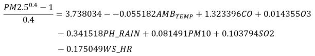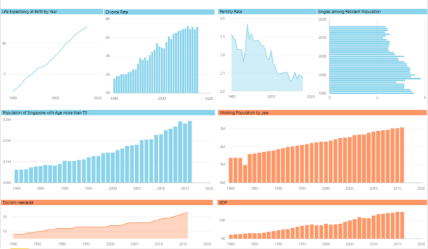The shortage of healthcare professionals is expected to keep increasing, and if nothing is done, the shortage of doctors is expected to reach 5504 in 10 years’ time while the shortage of nurses is approximately 9100 in year 2027.

How does the proportion of doctors and nurses in Singapore compare with other countries?

The proportion of doctors in Singapore is fourth among the six countries compared. Although the proportion of doctors in Singapore is only slightly higher than the proportion of doctors in Japan and Korea, it is much less than the proportion of doctors in Israel. In terms of nurses, Singapore is also in the middle of the list, higher proportion than Korea and Israel but lower than Japan – an aging developed country and UK and USA.

 What strategies can we take to increase the Healthcare workforce in Singapore?

We investigated the origins of the healthcare professionals in Singapore, and where they were trained. The number of healthcare professionals who are trained locally is fairly stable. This makes sense, as the capacity of the universities for medicine in Singapore is a limiting factor. One possibility is to increase local supply by starting a new medicine school and further increasing intakes of local medicine and nursing schools. The other direction is to attract more overseas trained professional.

Data Sources

MOH Statistics
https://www.moh.gov.sg/content/moh_web/home/statistics.html
Data.gov.sg
https://data.gov.sg/group/health
World Bank Healthcare Indicators
http://data.worldbank.org/indicator/SH.MED.PHYS.ZS?page=5
Singapore Nursing Board Reports
http://www.healthprofessionals.gov.sg/content/hprof/snb/en/topnav/publications_forms/publications.html
Singapore Medical Council Reports
http://www.healthprofessionals.gov.sg/content/hprof/smc/en/topnav/publication.html

Team Members

Huang Wei  (A0163367Y)
Lwi Tiong Chai  (A0163298U)
Meng Yang   (A0163427E)
Quan Yu  (A0049495N)
Tan Xinli Steven  (A0052121A)

Infocomm Industry’s Manpower Supply and Demand in Singapore

The infocomm industry has been a key economic sector in Singapore ever since the 1980s. In recent years, it has grown rapidly, especially after the smart nation initiative was announced in 2014.

As with all industry sectors, there is a need to gauge demand and tailor the supply of trained manpower in order to take advantage of growth. Too little supply of skilled labor and the industry’s growth will be stunted, reducing the benefits to the nation and population. Too much and there’s a risk of structural unemployment.

With this in mind, we present a dashboard using data from Data.gov.sg, consolidating various datasets on the infocomm industry, workforce numbers , and details on university graduates

Goals

This dashboard is for the MOM planning team director, and will give him/her a birds-eye view of the infocomm industry’s manpower supply and demand in Singapore, as well as present information that will facilitate effective decision-making with regards to meeting the manpower needs of the infocomm industry.

Questions

This dashboard will enable the director to answer the followng questions:

1. Is the infocomm industry growing in Singapore?
2. What are the main characteristics of Singapore’s infocomm workforce?
3. What are the main trends that Singapore’s infocomm workforce are facing?
4. Does Singapore have enough skilled workers for the growing infocomm industry?
5. What are the most effective ways to tackle this skills and demand shortage, if any?

Metrics

The metrics will encompass the growth of the infocomm industry in Singapore, the supply, demand, and characteristics of Singapore’s infocomm workforce, and the characteristics of fresh graduates in Singapore.

1. Infocomm industry worker numbers over time
2. Graduates in IT domain by year
3. Vacancies by year
4. Age distribution of Singapore’s infocomm workforce
5. Gender distribution of Singapore’s infocomm workforce
6. Residential status distribution of Singapore’s infocomm workforce
7. Qualification
8. Graduation disciplines

Dashboard

Insights

From the dashboard, one can see some bright spots with regards to Singapore’s infocomm manpower situation. ​

Firstly, the total vacancy rate has decreased, with vacancies remaining constant while the number of infocomm workers have increased​. This means that infocomm manpower planning is working well, meeting the demands of companies without much vacancies or excess.

Also, the skill level of infocomm professionals has increased, with more graduates and less diploma holders. ​This bodes well for Singapore’s infocomm sector, making it easier for companies to incorporate advanced technologies in AI and machine learning, for example.

​That said, there is much to be improved​ as well. To start with, there is a distinct lack of fresh young infocomm talent in Singapore​. As older professionals retire or move to managerial positions, there will exist a skills gap that will need to be filled. This problem will have to be solved by concentrating efforts in recruitment at the university level​, by marketing the infocomm sector as a hip one full of opportunities.

Next, the number of non-resident infocomm workers has increased relative to that of locals, signifying that local professionals not stepping up to work in the infocomm sector​. Here, relevant agencies can seek to improve awareness of opportunities in the infocomm sector​ among locals, as well as establish training programs to improve the skill base, based on the current Skillsfuture program.

Lastly, women only make up one-third of the total​ infocomm workforce. While this gender gap does not seem large, the proportion has stayed constant through the years, indicating that there may be a hidden systemic reason why women are not as well-represented in the industry. In this case, it may be possible to run campaigns to attract women into the infocomm sector​.

References

Employed ICT Manpower​
https://data.gov.sg/dataset/employed-ict-manpower​
​
Infocomm Manpower by Residential Status, Highest Qualification ​Attained, Gender, Discipline of Study and Age​
https://data.gov.sg/dataset/infocomm-manpower​
​
​Graduates From University First Degree Courses By Type Of Course​
https://data.gov.sg/dataset/graduates-from-university-first-degree-courses-by-type-of-course​
​
Infocomm Manpower Vacancies​
https://data.gov.sg/dataset/infocomm-manpower-vacancies​

Team Members

LIU Huan​
LIU Rui​
MA Ben​
NG Yee Siang Terence​
SHEN Yaoxin

Singapore Tourism Board Targeted Marketing Strategy

Business Goals

• Target Audience

This presentation is tailored for the Director of Marketing in Singapore Tourism Board. Whose role is to formulate and implement new marketing strategies to promote Singapore as a compelling destination for international visitors.

• Goal

Tourism is a major contributor to Singapore’s Economy. Given the competitive landscape where destinations in the region and around the world are stepping up their investments to attract visitors. Our main goal is to profile international visitors coming to Singapore to gain a deeper understanding on their needs and preferences when they are in Singapore. This is to facilitate creating a more targeted and cogent Marketing Plan tailor made to each individual Country. This will potentially lead to better yield in attracting new visitors to Singapore or stay in Singapore longer for every marketing dollar spend.

Questions

To better guide the formulation of the Market Strategy, We generalised the problem space into 5 Questions that we seek to answer.

1.Which are the Top Countries of Origin for International Visitor Arrivals?
We want to identify the distribution of countries from which Singapore’s visitors come from. This is to provide a general sense of the current landscape of visitorship.

2.When are the International Visitors coming to Singapore?
We wish to identify any seasonal patterns of visitor arrivals (monthly). This is to identify optimal timings for running promotions and marketing events to attract visitors to Singapore.

3.Where do International Visitors visit in Singapore?
We want to get a general sense of tourism attractions that the visitors visited in Singapore.

4.What are the types of Attractions that International Visitors will usually visit?
This is to get a more specific view on the visitorship pattern on free and paid attractions. This is to retrieve more targeted insights.

5.Where do International Visitors spend their money on?
We want to observe what the visitors are spending their money on in Singapore as this will provide a glimpse of their preferences and possible income levels.

Metrics

1.Annual International Visitor Arrivals by Country of Residence

2.Monthly International Visitor Arrivals by Country of Residence

3.Paid and Free Access Attractions and Sites Visited Yearly

4.Shopping Items Purchased in terms of Popularity Yearly

Data Collection

We collected open source datasets primarily from 2 sources – www.data.gov.sg and STB Annual Report. From the mentioned sources we acquired 5 years (2011 to 2015) worth of data pertaining to International Visitors Arrival Statistics and Shopping Items Purchased in Terms of Popularity etc.

Dashboard

Visualization Overview

1. Top Arrivals By Country
The Top Arrivals are visualized with a Geographical Map. This visualization provides an overview of where are the countries of origin for the international visitors to Singapore. We want to establish a view of the current landscape of visitorship.

2. Average Monthly Arrivals (Top 5 Countries)
The Average Monthly Arrivals from the dataset is visualized in a line chart with the X axis being the Month of the Year and the Y Axis being the Average Number of Arrivals. We want to identify any seasonal patterns in visitor arrivals by country.

3. Top 5 Attractions (Paid / Free)  Visited
The Top 5 Paid Attractions and Top 5 Free Attractions are displayed with a radar chart. We want to gain an understanding of the activities of the visitors here. In this visualization we filtered the visualization to show only the activities of the visitors from the Top 5 Country of Arrivals.

4. Top 5 Popular Spending Items
The Popular Spending Items is visualized in a Clustered Column chart, where the various categories of spending items are grouped according to the visitors from a particular country. We want to identify where the visitors will usually spend their money on in Singapore.

Insights

Seasonality Patterns

 

There is a spike in tourist arrivals from Indonesia in the month from November to December. The Indonesians may be likely to be attracted to the Christmas festivities in Singapore. Likewise a similar observation can be seen for China Visitors for the month of June to July. This time frame coincides with Great Singapore Sale event happening.

Preference for Places with Strong Ethnic Identities

In the Radar Chart for Attractions, we observe that apart from the highest ranked Orchard Road (Free) and MBS (Paid) (Both are already famous landmarks in Singapore). Ranked after Orchard Road is actually Chinatown and Little India, both these places have a strong ethnic heritage that seem to be attractive to our visitors. The hypothesis that we can generate from this is that these are the places that resonate with foreigners who wants to know more about the cultural aspect of Singapore.

Spending Patterns

Visitors mostly spent money on Fashion/Accessories as well as Confectionery / Food. One interesting observation is that for visitors from China they are more likely to spent on Cosmetics/Healthcare and Food which is unlike the rest of the visitors. This seem to indicate that for marketing Singapore as a place for healthcare may appeal more to the Chinese population than the usual “shopping heaven” tagline which Singapore is associated with.

Recommendations

• Marketing Activity Timing
  Time the Marketing Activities of each individual country in prior months of lull periods leading up to Peak Season for each country. This may increase the probability of new visitors going to Singapore as these Peak periods may coincide with holiday periods in their respective Countries.
• Curate Advertorial Material to Popular Locations
  Specially select landmarks or key attractions that tourist from a certain country is known to visit. For example, as identified in 1 of the insights Places like Chinatown and Little India are popular with visitors from certain countries. It will be a good idea to include pictorials of these places into marketing materials as part of the marketing plan. These may resonate better with the targeted audience.
• Retail Partnership Promotion
  Create special promotional shopping events with local retailers based on insights gathered from the Visitor’s spending patterns. For example, STB can partner local retailers to market Singapore to the population in China, they can offer special discount vouchers to popular items that Chinese citizens will always buy in Singapore.  By bundling these offers on top of Marketing Singapore as a whole, may have a higher chance of enticing visitors to come over.

DataSources

• Singapore Tourism Statistics from 2011 to 2015
  https://www.stb.gov.sg/statistics-and-market-insights/Pages/statistics-Annual-Tourism-Statistics.aspx
• Visitor International Arrivals to Singapore Monthly by Country
  https://data.gov.sg/dataset/total-visitor-international-arrivals-to-singapore?resource_id=83063203-ff81-4764-a9dc-c4e209921fe7
  

 

Team Members (Team 02):

Tan Boon Leong (E0147023)
Wu Hua Qing (E0146888)
Sudarsan Pula (E0146762)
Mai Dong Hua (E0146993)
Woo Chia Wei (E0146920)

Singapore Crime Rate Analysis

Singapore is among one of the safest countries in the world. Overall crime rate in Singapore is very less. The Singapore Police Force (SPF) ensures to maintain safety and harmony in country. The SPF makes every effort to provide precise and dependable data, made with the intent to accurately depict current trends. It is important to analyze the crime rate as it will help to determine the preventable crimes and more efforts can be put in that area. Getting information such as regions most affected and the gender & age group most affected will help to determine the methods and plans implementation strategy.
We have collected information regarding Singapore crime rate from publicly available sources. The primary data set is overall crime rate data from 2008 to 2015 from Singapore government data website. We cross-referenced this data with the age group of victims, gender of the victims, overall preventable crimes and crime rate per police division based on region.

Goal:
To analyze crime rate in Singapore to study categories of the most recurring crime, locations most impacted and types of preventable crimes over time and across the genders per police division for Singapore Police Force Chief.

 

Questions:

Is there an increase in the overall crime rate over the years?

As per the analysis crime rate has not increased over time based on the data, in fact it is recorded that in 2010 the crime rate was maximum and then decreased gradually till 2013. The year 2013 recorded the least crime rate after which it started to increase again but never reached the maximum point of 2010. There is decrease in the Theft and related crimes. From year 2013, there is increase in the commercial crimes. Commercial crimes are mostly related to the e-transactions. Due to this the overall crime rate is increasing from 2013 to 2015.

What is the most reoccurring type of crime?

Theft and related crimes are the most reoccurring crime over the entire time period. Even though there is a gradual decrease in theft and related crimes from 2010 to 2015 it still remains the most recurring crime. Commercial crimes were low and almost constant till 2013 and there was a sharp increase. In year 2015, commercial crimes are noted at its peak.

What is the most reoccurring type of preventable crime?

Preventable crimes are the ones which can be controlled even before they occur.Outrage of modesty is the most reoccurring preventable crime over the entire time period and across all the regional police divisions followed by theft.

Which gender is the most affected over time?

As per the analysis the gender most affected over time changes as per the type of crime i.e. Women were mostly affected by cheating and outrage of modesty where as Men were mostly impacted by riots, robbery and serious hurt.

Which age group is the most impacted?

People above the age group of 21 years i.e. adults are mostly the victims of different types of crimes over the time period. In the victims children and youth are not in great numbers.

Which region is the most impacted by preventable type of crimes?

Bedok region was most impacted by different types of preventable crimes like snatch theft, outrage of modesty over the entire time period. Central police division is least affected by preventable type of crimes.

Which is the least occurring crime?

As per the analysis it was observed that murder was the least occurring crime followed by rape. Violent or serious crimes and housebreaking are among the least occurring  crimes.

Metrics (KPI):

1. Overall Crime Rate
2. Age wise crime rate
3. Gender wise crime rate
4. Location wise crime rate
5. Preventable crime rate

 

Conclusion:

The maximum amount of crime rate was recorded during the year 2010, with Theft being the most recurrent crime and outrage of modesty being the most recurrent preventable crime. In the year 2013 the least crime rate was recorded, after which there is a gradual increase till 2015; though it has not reached the peak recorded in year 2010. Serious crimes like murder and rape are very low throughout the tenure. Bedok police division recorded highest number of preventable crimes.

Link to view the Dashboard on Tableau Public:  

https://public.tableau.com/views/singapor-crime_analysis/OverallCrimeAnalysis?:embed=y&:display_count=yes&publish=yes

Team Members:  Sowndarya Satya  (A0163229E), Suma Mulpuru (A0163231U), Swamini Wadekar (A0163337E),Nandha Kumar  (A0163346E)

 

Data Sources:

Overall Crime rate:
https://data.gov.sg/dataset/overall-crime-cases-crime-rate?view_id=4e163b21-679e-48e8-a9dd-38de1239f940&resource_id=56987172-00a3-4f0c-be4f-12f3e7ec4e1aPreventable crimes:
https://data.gov.sg/dataset/five-preventable-crime-cases-recorded-by-npcs?view_id=f96ca2b4-4156-46cc-b7ea-0b5b11f67e55&resource_id=10a2b502-2ffd-4df7-8b6f-6ea7d74893b7

Crime data:
https://data.gov.sg/dataset/overall-crime-cases-crime-rate?view_id=b65b0741-3dfb-4563-ad40-394cf6dbd819&resource_id=efc3dd2a-8779-46be-b8c7-882712d49451

Victims of selected major selected offences by age group:  https://data.gov.sg/dataset/victims-of-selected-major-selected-offences?view_id=b78f9084-c3f2-41d2-814b-01c9e4258a27&resource_id=b71a68b2-e059-4af3-a084-25ac73cab811

Police force division:
https://data.gov.sg/dataset/singapore-police-force-npc-boundary

 

 

 

 

An American Improving Academic Customer Library Relations with Social Listening: A Case Study of an American Academic Library

ABSTRACT
Strategic social media plays a crucial role in contemporary customer relationship management (CRM); however, the best practices for social CRM are still being discovered and established. The ever-changing nature of social media challenges the ability to establish benchmarks; nonetheless, this article captures and shares actions, insights, and experiences of using social media for CRM. This case study examines how an academic library at a mid-size American university located in northeast Florida uses social media to engage in social listening and to enhance CRM. In particular, the social listening practices of this library are highlighted in relation to how they influence and potentially improve CRM. By exploring the practices of this single institution, attempts are made to better understand how academic libraries engage with customers using social media as a CRM tool and ideas for future research in the realm of social media and CRM practices are discussed.
Keywords:
Academic Library, Customer Relationship Management, Facebook, Hashtags, Instagram, Library Customers, Social CRM, Social Media, Strategic Social Listening, Thomas G. Carpenter Library, Twitter

SOURCE: http://www.igi-global.com.libproxy1.nus.edu.sg/gateway/article/172050

SUBMITTED BY:  Ding Renzhi A0163220X, Gu Zhuyi A0163219H

                                  Ma Min A0163305N, Gao Ruofei A0163436E

                                  Zheng Weiyu A0163412R

Managing Customer Loyalty through Acquisition, Retention and Experience Efforts: An Empirical Study on Service Consumers in India

Recent developments in the marketing literature highlight the significance of consumer relationship management (CRM) in driving consumer loyalty (CL). In order to provide a clear understanding of the impact of CRM on CL, this study develops an integrated framework of CRM activities: Acquisition, retention, and experience to manage Customer Loyalty through direct and indirect approaches (with the mediation of satisfaction, trust, and commitment). The article utilizes a survey-based empirical study of 600 consumers from three service sectors (health, retail, and wellness). The findings of the study suggest that a firm that pays more attention to manage consumer experiences would be significantly benefited from the implementation of CRM programs. Consumer experience efforts have the positive impact on CL through commitment in all three sectors. Service manager should have clarity and consciousness that consumers are not looking for just traditional CRM benefits such as value proportion, reward points and so on but specifically seek for a pleasant experience of various touchpoints. Various frameworks of acquisition of CRM activities to manage Customer Loyalty has been analyzed.

Key Words:
Consumer loyalty, Consumer relationship management, Consumer experience management, Satisfaction, Trust, Commitment

Source : Managing Consumer Loyalty through Acquisition, Retention and Experience Efforts: An Empirical Study on Service Consumers in India

Submitted by TEAM MARS

1. Mutharasan Anbarasan(A0163257A)
2. Raghavan Kalyanasundaram(A0163316L)
3. Saravanan Kalastha Sekar(A0163309H)
4. Seshan Sridharan(A0148476R)
5. Sindhu Rumesh Kumar(A0163342M)

Customer Churn Prediction in the Telecommunications Sector Using Rough Set Approach

This study aims to develop an improved customer churn prediction technique, as high customer churn rates have caused an increase in the cost of customer acquisition. This technique will be developed through identifying the most suitable rule extraction algorithm to extract practical rules from hidden patterns in the telecommunications sector.

Submitted by:
Arun Kumar Balasubramanian
Devi Vijayakumar
Sunil Prakash
Gaelan Gu
Sambit Kumar Panigrahi